Getting started with BLISS
This page will present what is the BLISS control system and how to start using it.
BLISS presentation
BLISS control system provides a global approach to run synchrotron experiments requiring to synchronously control motors, detectors and various acquisition devices thanks to hardware integration, Python sequences and an advanced scanning engine.
As a Python package, BLISS can be easily embedded into any Python application and data management features enable online data analysis. In addition, BLISS ships with tools to enhance scientists user experience and can easily be integrated into TANGO based environments, with generic TANGO servers on top of BLISS controllers.
On user point of view, BLISS presents different aspects:
- BLISS shell: a command line interface to interact with devices and to run sequences
- Sequences programming to create customized experiments
- Configuration of all devices involved in the experiments
BLISS shell
BLISS comes with a command line interface based on ptpython.
BLISS uses the concept of session to allow user to define a set of procedures and devices to use in a particular circumstance (like alignment, specific hutch or specific experiment).
bliss -s eh1
                       __         __   __
                      |__) |   | /__` /__`
                      |__) |__ | .__/ .__/


Welcome to BLISS version 0.01 running on pcsht (in bliss Conda environment)
Copyright (c) 2015-2019 Beamline Control Unit, ESRF
-
Connected to Beacon server on pcsht (port 3412)
eh1: Executing setup...
Initializing 'pzth`
Initializing 'simul_mca`
Initializing 'pzth_enc`
Done.

EH1 [1]:
The -s command line option loads the specified session at startup,
i.e. configuration objects defined in the session are initialized,
then the setup file is executed. Finally the prompt returns to user.
-h option allows to get an overview of other command-line features.
% bliss -h
Usage: bliss [-l | --log-level=<log_level>] [-s <name> | --session=<name>]
             [--no-tmux] [--tmux-debug]
       bliss [-v | --version]
       bliss [-c <name> | --create=<name>]
       bliss [-d <name> | --delete=<name>]
       bliss [-h | --help]
       bliss --show-sessions
       bliss --show-sessions-only

Options:
  -l, --log-level=<log_level>   Log level [default: WARN]
                                (CRITICAL ERROR INFO DEBUG NOTSET)
  -s, --session=<session_name>  Start with the specified session
  -v, --version                 Show version and exit
  -c, --create=<session_name>   Create a new session with the given name
  -d, --delete=<session_name>   Delete the given session
  -h, --help                    Show help screen and exit
  --no-tmux                     Deactivate Tmux usage
  --tmux-debug                  Allow debugging keeping tmux alive after
                                Bliss shell exits
  --show-sessions               Display sessions and tree of sub-sessions
  --show-sessions-only          Display available sessions names only
A session can be created using -c option:
% bliss -c eh1
creating 'eh1' session
Creating: /blissadm/local/beamline_configuration/sessions/eh1_setup.py
Creating: /blissadm/local/beamline_configuration/sessions/eh1.yml
Creating: /blissadm/local/beamline_configuration/sessions/scripts/eh1.py
Learn more about BLISS sessions
Examples of standard shell functions
Once BLISS shell is launched, user can use it as a typical python shell in addition to be able to act on configured devices.
Most common devices are counters and motors.
Most common actions a user would like to perform are counting and scaning.
Many standard functions are then provided to help user to perform such actions on such devices.
wa(): shows a table of all motors in the session, with positions.lscnt(): shows a table of all counters in the session.ascan(axis, start, stop, n_points, count_time): moves an axis from start to stop in n_points steps and counts count_time at each step.
Help
Help about BLISS functions can be accessed with help(<command_name>):
BLISS [2]: help(wa)
Help on function wa in module bliss.common.standard:

wa(**kwargs)
    Displays all positions (Where All) in both user and dial units
``


Learn more about other [standard shell functions](shell_std_func.md).

[Learn more about BLISS shell](shell_cmdline.md).


## Counters

First fundamental objects to consider in BLISS are the *counters*. A
counter is used to depict the reading of a device.

The most simple function to read all defined counters is
`ct(<counting_time>)`.

```python
DEMO [3]: ct(0.1)
Fri Jun 7  16:32:17 2018
   dt[s] = 0.0     (    0.0/s)
  simct1 = 0.50109 ( 5.0109/s)
  simct2 = 0.49920 ( 4.9920/s)
  simct3 = 0.50403 ( 5.0403/s)
  simct4 = 0.50311 ( 5.0311/s)

  Out [3]: Scan(name=ct_1, run_number=1)
To use only a sub-set of counters, they have to be specified in argument:
DEMO [5]: ct(1, simct1, simct4)

Fri Nov 16 16:37:43 2018

   dt[s] = 0.0    (    0.0/s)
  simct1 = 0.49872 ( 0.49872/s)
  simct4 = 0.50021 ( 0.50021/s)
  Out [20]: Scan(name=ct_3, run_number=3)
Using measurement groups
An alternative of specifying counters for each scan is to rely on measurement groups.
DEMO [1]: align_counters
  Out [1]: MeasurementGroup:  align_counters (default)

           Enabled  Disabled
           -------  -------
           simct1
           simct2
           simct3
The measurement group can be passed to a scan or ct procedure to
define counters for the scan:
DEMO [4]: ascan(simot1, -2, 2, 7, 0.1, align_counters)

Scan 5 Wed Feb 21 15:26:31 2018 /tmp/scans/demo/ demo user = guilloud
ascan simot1 -2 2 7 0.1

        #         dt(s)        simot1        simct1        simct2        simct3
        0       4.18972            -2      0.501319     0.0165606    0.00511711
        1       5.12933         -1.33      0.728287     0.0236184     0.0073165
        2       6.06347         -0.67      -0.33863      0.257847      0.251785
        3       6.98862             0     -0.608677       1.01518      0.997982
        4       7.92987          0.67      -2.29062      0.261047      0.249959
        5       8.86126          1.33      0.219424      0.023286     0.0137307
        6       9.78928             2     -0.558003    0.00988632     0.0165549

Took 0:00:09.993863
Multiple measurement groups can be passed:
DEMO [20]: print MG1.available, MG2.available   #  4 counters defined in 2 MG
['simct2', 'simct3'] ['simct4', 'simct5']

DEMO [21]: timescan(0.1, MG1, MG2, npoints=3)

Scan 15 Wed Feb 21 16:31:48 2018 /tmp/scans/demo/ demo user = guilloud
timescan 0.1

        #         dt(s)        simct2        simct3        simct4        simct5
        0     0.0347409       0.50349      0.494272      0.501698      0.496145
        1       0.13725       0.49622      0.503753      0.500348      0.500601
        2        0.2391      0.502216      0.500213      0.494356      0.493359

Took 0:00:00.395435
Active measurement group
If no counter and no measurement group is specified to the scan command, a default one is used: the active measurement group. Indeed, there is always only one active measurement group at a time.
ACTIVE_MG is a global variable to know the active measurement group:
 DEMO [1]: ACTIVE_MG
   Out [1]: MeasurementGroup:  align_counters (default)

             Enabled  Disabled
             -------  -------
             simct2
             simct3
The active measurement group is the one used by default by a scan or a ct:
DEMO [32]: ct(0.1)

Wed Feb 21 15:38:51 2018

   dt(s) = 0.016116142272 ( 0.16116142272/s)
  simct2 = 0.499050226458 ( 4.99050226458/s)
  simct3 = 0.591432432452 ( 5.91432432452/s)
The set_active() method can be used to change the active measurement group:
DEMO [33]: ACTIVE_MG
  Out [33]: MeasurementGroup:  align_counters (default)

                 Enabled  Disabled
                 -------  -------
                 simct1
                 simct2
                 simct3

    DEMO [34]: MG2.set_active()

    DEMO [35]: ACTIVE_MG
      Out [35]: MeasurementGroup:  MG2 (default)

                  Enabled  Disabled
                  -------  -------
                  simct4
                  simct5
Note
The default active measurement group is the last defind in config.
Learn more about measurement groups.
Motors
Second fundamental objects to consider in BLISS are the motors.
Motors are used to reflect a change of a device. It can be an object movement or a device set-point.
Motors main parameters are:
- user and dial positions (potentially differing by an offset and a sign)
- velocity and acceleration
- high_limit and low_limit
wa() standard command is provided to show positions of all motors
defined in the current session.
DEMO [21]: wa()
Current Positions (user, dial)

simot1    simot2    simot3    simot4    simot5
--------  --------  --------  --------  --------
2.00000   4.00000   6.00000   8.00000   9.00000
2.00000   4.00000   6.00000   8.00000   9.00000
wm([motor]+) shows dial, limits and offset in addition to positions of one or
many motors.
To use only a sub-set of motors, they have to be specified in argument:
DEMO [24]: wm('simot1', 'simot4')
           simot1    simot4
-------  --------  --------
User
 High     10.00000  10.00000
 Current   2.00000   8.00000
 Low     -10.00000 -10.00000
Offset    -1.00000   4.00000

Dial
 High     11.00000   6.00000
 Current   3.00000   4.00000
 Low      -9.00000 -14.00000
Learn more about IcePap motors configuration.
Learn more about motor usage.
Basic scans
To perform a realistic acquisition, counters and motors have now to be used simultaneously. This is done using scans.
BLISS relies on a powerful scanning engine based on the principle of an acquisition chain, i.e. a tree of master and slave devices: master devices trigger acquisition, whereas slave devices take data. Complex acquisition chains can be built to perform any kind of data acquisition sequence. Read more about the BLISS scanning engine
The acquisition chain for each scan has to be provided by the user. In order to help with simple scans, BLISS provides a default acquisition chain to perform scans similar to the default, step-by-step, ones in Spec.
Default step-by-step scans
BLISS provides functions to perform scans a user would need for usual step-by-step measurements.
Most common are :
ascan(axis, start, stop, n_points, count_time, *counters, **kwargs)dscan: same asascan, withstart,stopas relative positions to current axis positiona2scan: same as ascan but with 2 motorsmeshto makes a grid using 2 motorstimescanto count without moving a motor
All scans can take counters in the arguments list. This is to limit the scan to the provided list of counters.
More about default scans.
ascan
ascan example with 1 motor and 2 counters.
TEST_SESSION [1]: ascan(roby, 0, 10, 10, 0.1, diode, diode2)

Scan 1 Wed Apr 18 08:46:20 2018 /tmp/scans/ test_session user = matias
ascan roby 0 10 10 0.1

    #         dt(s)          roby        diode2         diode
    0     0.0341308             0       5.88889       7.44444
    1      0.298563        1.1111      -2.88889      -6.88889
    2      0.529942        2.2222           -34       1.33333
    3      0.761447        3.3333      -30.1111      -11.7778
    4       1.00202        4.4444      -6.22222       11.3333
    5       1.23181        5.5556           -17      -5.11111
    6       1.46598        6.6667       12.5556      -8.44444
    7       1.69842        7.7778     -0.777778      -6.55556
    8       1.92679        8.8889      -10.5556            34
    9       2.16557            10            18      -25.5556

Took 0:00:02.328219
One-shot acquisition with integration time
The ct(time_in_s, *counters) function counts for the specified
number of seconds. It is equivalent of a timescan with npoints set
to 1.
Scan saving
The SCAN_SAVING global is a structure to tell BLISS where to save scan data:
ID29 [1]: SCAN_SAVING
 Out [1]: Parameters (default)
            .base_path      = '/users/blissadm/scans'
            .date_format    = '%Y%m%d'
            .template       = '{session}/{date}'
            .user_name      = 'opid29'
            .writer         = 'hdf5'
Find more info about how to use it in SCAN_SAVING section
Retrieving scan data
The get_data() function takes a scan object and returns scan data in
a numpy array. Scan data is retrieved from redis. Data
references are not resolved, which means 2D data is not returned.
Example:
TEST_SESSION [4]: myscan = ascan(roby, 0, 1, 10, 0.001, diode,
                                 simu1.counters.spectrum_det0, return_scan=True)
Activated counters not shown: spectrum_det0

Scan 3 Fri Apr 20 11:26:55 2018 /tmp/scans/test_session/
                                test_session user = matias
ascan roby 0 1 10 0.001

       #         dt(s)          roby         diode
       0      0.337308             0            83
       1      0.759228        0.1111           -10
       2       1.17105        0.2222            57
       3       1.58996        0.3333            43
       4       2.00024        0.4444           -44
       5       2.41497        0.5556           -16
       6       2.83309        0.6667           -74
       7       3.23919        0.7778            18
       8       3.65932        0.8889            74
       9       4.07872             1           -43

Took 0:00:04.441955

TEST_SESSION [5]: data = get_data(myscan)
The numpy array is built with fields, it is easy to get data for a particular column using the counter name:
TEST_SESSION [8]: data['diode']
         Out [8]: array([ 83., -10., 57., 43., -44., -16., -74., 18., 74., -43.])
Online data display
Online data display relies on Flint, a graphical application shipped with BLISS and built on top of silx.
Flint can be started automatically when a new scan begins, by
configuring SCAN_DISPLAY:
SCAN_DISPLAY.auto = True
Plots are displayed in the Live tab. Depending on the scan acquisition chain, 3 types of plots can be shown:
- 1D plots, showing curves from the scan scalar counters
- 1D spectra, showing 1D scan counters (like MCA)
- 2D images, showing 2D data counters (typically, Lima detectors data)
Plots are grouped by the topmost master, i.e. as long as the number of points for a master corresponds to its parent, the plots are attached to this master (recursively, up to the root master if possible). If number of points diverges between 2 masters, then underlying data is represented in another set of plot windows. So, there is no limit to the number of windows in the Live tab, it depends on the scan being executed.
Note
2D images are always represented in their own plot window.
Live scan data in Flint
TEST_SESSION [8]: SCAN_DISPLAY.auto=True

TEST_SESSION [9]: timescan(0.1, lima, diode, diode2, simu1.counters.spectrum_det
         ...: 0, npoints=10)
Activated counters not shown: spectrum_det0, image

Scan 145 Wed Apr 18 11:24:06 2018 /tmp/scans/ test_session user = matias
timescan 0.1

       #         dt(s)        diode2         diode
       0     0.0219111       12.5556      -9.33333
       1      0.348005        30.625         0.125
       2      0.664058       2.88889      -10.2222
       3      0.973582       7.11111       8.44444
       4       1.28277       21.7778       36.3333
       5       1.59305      -15.8889             5
       6       1.90203       43.4444       19.4444
       7       2.21207       20.7778       11.6667
       8       2.52451      -7.88889       24.2222
       9       2.83371        24.125         7.625

Took 0:00:03.214453

TEST_SESSION [9]:
Flint screenshot:

Read more about Online Data Display
BLISS as a library
BLISS is primarily a Python library, thus BLISS can be embedded into any Python program.
BLISS is built on top of gevent, a coroutine-based asynchronous networking library. Under the hood, gevent works with a very fast control loop based on libev (or libuv).
The loop has to be running in the host program. When BLISS is imported, gevent monkey-patching is applied automatically (except for the threading module). In most cases, this is transparent and does not require anything from the host Python program.
Note
When using BLISS from a command line or from a graphical interface, gevent needs to be inserted into the events loop.
For example a BLISS-friendly IPython console can be started like this:
python -c "import gevent.monkey; gevent.monkey.patch_all(thread=False); import IPython; IPython.start_ipython()"
The line above launches Python, makes sure Python standard library is patched, without replacing system threads by gevent greenlets (which seems like a reasonable option), then starts the IPython interpreter.
From now on it is possible to use BLISS as any Python library:
    In [1]: from bliss.common.axis import Axis

    In [2]: from bliss.controllers.motors import icepap

    In [3]: ice = icepap.Icepap("iceid2322", {"host": "iceid2322"},
                               [("mbv4mot", Axis,
                               {"address":1,"steps_per_unit":817,
                               "velocity": 0.3, "acceleration": 3
                               })], [], [], [])

    In [4]: ice.initialize()

    In [5]: mbv4 = ice.get_axis("mbv4mot")

    In [6]: mbv4.position()
    Out[6]: 0.07099143206854346

    In [7]:
The example above creates an IcePAP motor controller instance,
configured with a mbv4mot axis on IcePAP channel 1. Then, the
controller is initialized and the axis object is retrieved to read the
motor position.
Note
This example is meant to demystify BLISS – the only recommended way to use BLISS is to rely on BLISS Beacon to get configuration and to use the BLISS shell as the preferred command line interface.
Interacting with plots
BLISS provides tools to interact with plot windows in Flint. Each
scan object has a .get_plot() method, that returns a Plot
object. The argument to pass to .get_plot is a counter – thus, the
plot containing this counter data is returned:
TEST_SESSION [8]: s = loopscan(5, 0.1, lima, return_scan=True)
Activated counters not shown: image

Scan 2 Wed Apr 18 11:36:11 2018 /tmp/scans/test_session/
                                test_session user = matias
timescan 0.1

       #         dt(s)
       0      0.959486
       1        1.0913
       2       1.23281
       3       1.36573
       4       1.50349

Took 0:00:01.666654

TEST_SESSION [9]: p = s.get_plot(lima)
TEST_SESSION [10]: p
         Out [10]: ImagePlot(plot_id=2, flint_pid=13678, name=u'')
Starting from the ImagePlot object, it is possible to ask user for
making a rectangular selection for example:
TEST_SESSION [11]: p.select_shape("rectangle")
BLISS shell is blocked until user makes a rectangular selection:
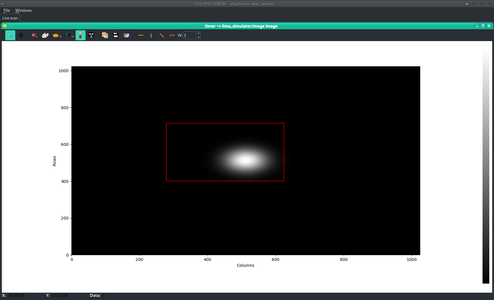
Then, result is returned by the .select_shape method:
Out [11]: ((278.25146, 716.00623), (623.90546, 401.82913)